California housing regression
In this notebook we’ll use the ITEA_regressor to search for a good expression, that will be encapsulated inside the ITExpr_regressor class, and it will be used for the regression task of predicting California housing prices.
[1]:
import numpy  as np
import pandas as pd

import matplotlib.pyplot as plt

from sklearn import datasets

from sklearn.model_selection import train_test_split
from IPython.display         import display

from itea.regression import ITEA_regressor
from itea.inspection import *

import warnings
warnings.filterwarnings(action='ignore', module=r'itea')
The California Housing data set contains 8 features.
In this notebook, we’ll provide the transformation functions and their derivatives, instead of using the itea feature of extracting the derivatives using Jax.
Creating and fitting an ITEA_regressor
[2]:
housing_data = datasets.fetch_california_housing()
X, y         = housing_data['data'], housing_data['target']
labels       = housing_data['feature_names']

X_train, X_test, y_train, y_test = train_test_split(
    X, y, test_size=0.33, random_state=42)

tfuncs = {
    'log'      : np.log,
    'sqrt.abs' : lambda x: np.sqrt(np.abs(x)),
    'id'       : lambda x: x,
    'sin'      : np.sin,
    'cos'      : np.cos,
    'exp'      : np.exp
}

tfuncs_dx = {
    'log'      : lambda x: 1/x,
    'sqrt.abs' : lambda x: x/( 2*(np.abs(x)**(3/2)) ),
    'id'       : lambda x: np.ones_like(x),
    'sin'      : np.cos,
    'cos'      : lambda x: -np.sin(x),
    'exp'      : np.exp,
}

reg = ITEA_regressor(
    gens         = 50,
    popsize      = 50,
    max_terms    = 5,
    expolim      = (0, 2),
    verbose      = 10,
    tfuncs       = tfuncs,
    tfuncs_dx    = tfuncs_dx,
    labels       = labels,
    random_state = 42,
    simplify_method = 'simplify_by_coef'
).fit(X_train, y_train)
gen | smallest fitness | mean fitness | highest fitness | remaining time
----------------------------------------------------------------------------
  0 |         0.879653 |     1.075672 |        1.153701 | 0min41sec
 10 |         0.794826 |     0.828574 |        0.983679 | 1min9sec
 20 |         0.791858 |     0.794191 |        0.802730 | 0min57sec
 30 |         0.785556 |     0.790837 |        0.892611 | 0min43sec
 40 |         0.773925 |     0.790826 |        1.024342 | 0min19sec
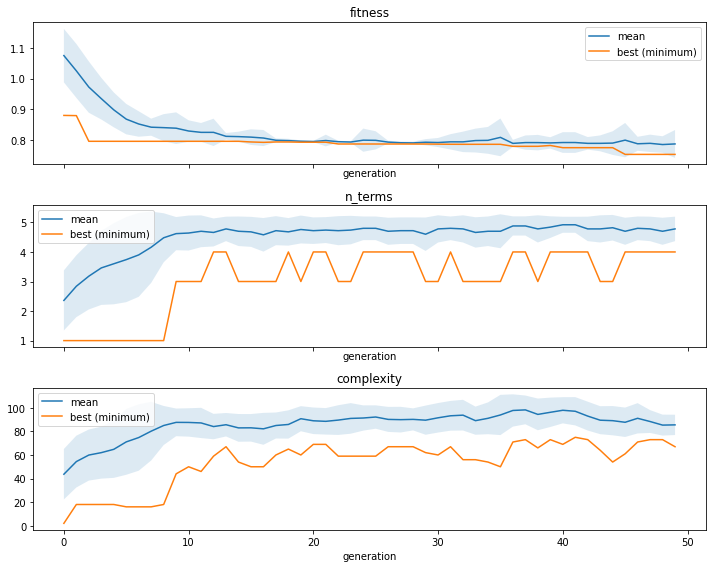
Inspecting the results from ITEA_regressor and ITExpr_regressor
We can see the convergence of the fitness, the number of terms, or tree complexity by using the ITEA_summarizer, an inspector class focused on the ITEA:
[3]:
fig, axs = plt.subplots(3, 1, figsize=(10, 8), sharex=True)

summarizer = ITEA_summarizer(itea=reg).fit(X_train, y_train)

summarizer.plot_convergence(
    data=['fitness', 'n_terms', 'complexity'],
    ax=axs,
    show=False
)

plt.tight_layout()
plt.show()
Now that we have fitted the ITEA, our reg contains the bestsol_ attribute, which is a fitted instance of ITExpr_regressor ready to be used. Let us see the final expression and the execution time.
[4]:
final_itexpr = reg.bestsol_

print('\nFinal expression:\n', final_itexpr.to_str(term_separator=' +\n'))
print(f'\nElapsed time: {reg.exectime_}')
print(f'\nSelected Features: {final_itexpr.selected_features_}')
Final expression:
 2.207*log(MedInc^2 * HouseAge * AveBedrms * Population^2 * Latitude) +
-0.901*log(HouseAge^2 * AveRooms^2 * Population^2 * AveOccup * Longitude^2) +
-1.392*log(MedInc^2 * AveRooms^2 * AveBedrms * Population^2 * Latitude^2 * Longitude^2) +
2.96*log(AveRooms * Longitude^2) +
0.0*sqrt.abs(MedInc^2 * AveRooms^2 * AveBedrms * Population * Longitude) +
-1.305

Elapsed time: 98.63136196136475

Selected Features: ['MedInc' 'HouseAge' 'AveRooms' 'AveBedrms' 'Population' 'AveOccup'
 'Latitude' 'Longitude']
[5]:
# just remembering that ITEA and ITExpr implements scikits
# base classes. We can check all parameters with:
print(final_itexpr.get_params)
<bound method BaseEstimator.get_params of ITExpr_regressor(expr=[('log', [2, 1, 0, 1, 2, 0, 1, 0]),
                       ('log', [0, 2, 2, 0, 2, 1, 0, 2]),
                       ('log', [2, 0, 2, 1, 2, 0, 2, 2]),
                       ('log', [0, 0, 1, 0, 0, 0, 0, 2]),
                       ('sqrt.abs', [2, 0, 2, 1, 1, 0, 0, 1])],
                 labels=array(['MedInc', 'HouseAge', 'AveRooms', 'AveBedrms', 'Population',
       'AveOccup', 'Latitude', 'Longitude'], dtype='<U10'),
                 tfuncs={'cos': <ufunc 'cos'>, 'exp': <ufunc 'exp'>,
                         'id': <function <lambda> at 0x7f9a607e9440>,
                         'log': <ufunc 'log'>, 'sin': <ufunc 'sin'>,
                         'sqrt.abs': <function <lambda> at 0x7f9a61057b00>})>
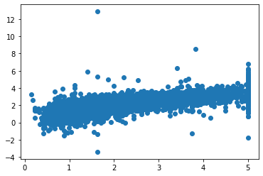
[6]:
fig, axs = plt.subplots()

axs.scatter(y_test, final_itexpr.predict(X_test))
plt.show()
We can use the ITExpr_inspector to see information for each term.
[7]:
display(pd.DataFrame(
    ITExpr_inspector(
        itexpr=final_itexpr, tfuncs=tfuncs
    ).fit(X_train, y_train).terms_analysis()
))
| coef | func | strengths | coef\nstderr. | mean pairwise\ndisentanglement | mean mutual\ninformation | prediction\nvar. | |
|---|---|---|---|---|---|---|---|
| 0 | 2.207 | log | [2, 1, 0, 1, 2, 0, 1, 0] | 0.021 | 0.459 | 0.567 | 13.738 |
| 1 | -0.901 | log | [0, 2, 2, 0, 2, 1, 0, 2] | 0.009 | 0.284 | 0.305 | 2.264 |
| 2 | -1.392 | log | [2, 0, 2, 1, 2, 0, 2, 2] | 0.015 | 0.501 | 0.681 | 7.419 |
| 3 | 2.96 | log | [0, 0, 1, 0, 0, 0, 0, 2] | 0.046 | 0.175 | 0.270 | 0.686 |
| 4 | 0.0 | sqrt.abs | [2, 0, 2, 1, 1, 0, 0, 1] | 0.0 | 0.357 | 0.603 | 0.168 |
| 5 | -1.305 | intercept | --- | 0.403 | 0.000 | 0.000 | 0.000 |
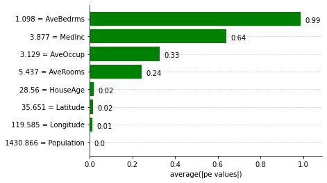
Explaining the IT_regressor expression using Partial Effects
We can obtain feature importances using the Partial Effects and the ITExpr_explainer.
[8]:
explainer = ITExpr_explainer(
    itexpr=final_itexpr, tfuncs=tfuncs, tfuncs_dx=tfuncs_dx).fit(X, y)

explainer.plot_feature_importances(
    X=X_train,
    importance_method='pe',
    grouping_threshold=0.0,
    barh_kw={'color':'green'}
)
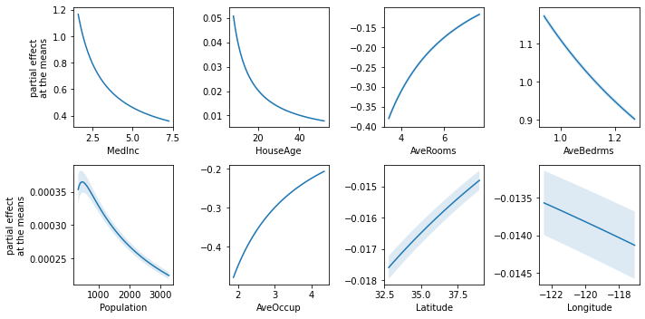
The Partial Effects at the Means can help understand how the contribution of each variable changes according to its values when their covariables are fixed at the means.
[9]:
fig, axs = plt.subplots(2, 4, figsize=(10, 5))

explainer.plot_partial_effects_at_means(
    X=X_test,
    features=range(8),
    ax=axs,
    num_points=100,
    share_y=False,
    show_err=True,
    show=False
)

plt.tight_layout()
plt.show()
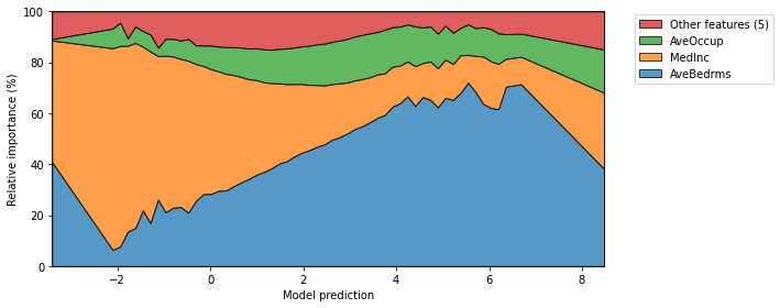
Finally, we can also plot the mean relative importances of each feature by calculating the average Partial Effect for each interval when the output is discretized.
[10]:
fig, ax = plt.subplots(1, 1, figsize=(10, 4))

explainer.plot_normalized_partial_effects(
    grouping_threshold=0.1, show=False,
    num_points=100, ax=ax
)

plt.tight_layout()